Data of the Age of Reptiles: Part 3 - Undercoat
Yale Peabody
R
Dinosaurs
Reconstructing the black and white undercoat of the Age of Reptiles mural.
Note
Originally published on January 02, 2018. Moved to new website on August 6, 2023 without edits.
Now that I have a few years more experience, it might be a good idea to revisit these ideas soon.
The Undercoat
Before Rudolph Zallinger painted the mural as we see it today, he painted the entire mural in “deliberately overmodeled” forms in black and white. This first coat is visible under the final colored mural, with the dark forms providing a three-dimensional effect.
Am I able to reconstruct this original undermodel using this low-resolution jpeg?
Reconstructing the undercoat
The best image of the original undercoat I have found is a portrait of Zallinger from 1944 where he is in the process of painting the shadowy undercoat. In the photo, the painting is visible starting at the Jurassic period with details extending through the Permian. For this analysis, I began with just the Jurassic and Triassic period for easy comparison.

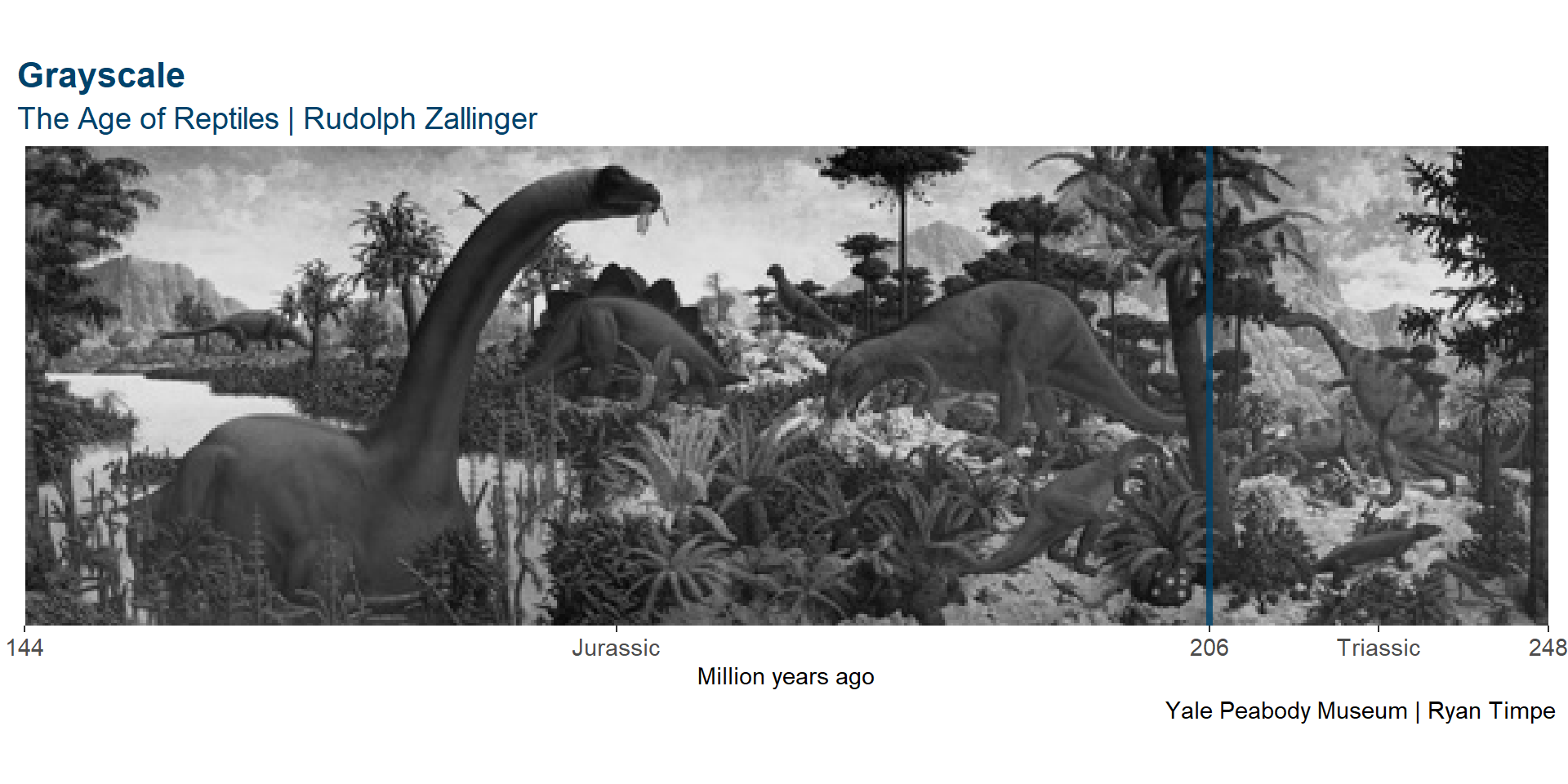
Grayscale
My first instinct to recreate the black and white undercoat was to convert the image to grayscale by assigning every color a darkness value between 0 and 1.
With a visual comparison of this image and the photo of the undercoat, it’s clear that this is not a good approach. The skies in particular stand out to me - in the final mural, the skies are the lightest areas in the final painting, but in the undercoat the upper portion of them is almost black. In contrast, the Allosaurus and Stegosaurus have white bodies in the undercoat and are rich dark colors in the final mural.
Shading by intensity
The undercoat layer provides the final painting with shadows for each element of the painting (animals, plants, terrain, sky, etc.). In order to recreate this layer, I need to differentiate between the elements in the painting. One way to do this is to split the painting by shades, and then run similar analyses independently on each one.

To get the groups, I square the grayscale values for each cells in order to further differentiate them, then allocate each shading intensity value into quintiles.
The lightest group contains mostly the skies while the darkest groups almost resemble the fauna in the undercoat. However, after a lot of trial and error, I was unable to come close to reconstructing the undercoat with this method.
Shading by color
Each object in the final mural was represented in the undercoat. I can’t (yet) easily split the mural into individual objects, however, for the most part, Zallinger used the undercoat to create various shades of the same color to paint each object. By splitting the mural into color types, I could come closer to recreating the undercoat.
After a lot of tweaking values and filtering steps, I came close to recreating the undercoat.
- I rounded each RGB channel into groups of the nearest 5% intensity.
- I turned these RGB channel values into color groups, determined by the relative intensity of R, G, B.
- How much more red than green is a pixel, more green than blue, and more red than blue.
- This grouping is important because a pixel with 100% each RGB is the same (but brighter) color as a pixel with 80% RGB.
- This created 88 unique color groups (not 20*20*20 = 8,000 because not all colors are in the painting.) Only 50 of these color groups are represented in more than 100 pixels.
- To ensure completely different colors are not grouped together (e.g. black and white), I further divided the color groups into 3 shadow groups: >90% brightness, 50-90%, and <50%.
- For each color * shadow group, only the pixels with a shadow value of at least 150% the minimum value are retained.
#Number of groups per RGB channel
color_group_n <- 20

chart.uc <- aor.shd.1 %>%
  mutate(Ru = R, Gu = G, Bu = B) %>%
  mutate_at(vars(Ru, Gu, Bu), funs(
    ifelse(. == 1, color_group_n-1, round(.*color_group_n))
  )) %>%
  mutate(
    del_RG = Ru - Gu,
    del_RB = Ru - Bu,
    del_GB = Gu - Bu
  ) %>%
  mutate(
    color_group = paste(del_RG, del_RB, del_GB)
  ) %>%
  select(-dplyr::starts_with("del_")) %>%
  mutate(shadow = ((1-R)+(1-G)+(1-B))/3) %>%
  mutate(shadow_group = case_when(
    shadow < 0.2 ~ "Light",
    shadow < 0.5 ~ "Medium",
    TRUE ~ "Dark"
  )) %>%
  group_by(color_group, shadow_group, period) %>%
  mutate(under = shadow > min(shadow)*1.5) %>%
  ungroup() %>%
  mutate_at(vars(R, G, B), funs(as.character(as.hexmode(.*255)))) %>%
  mutate_at(vars(R, G, B), funs(ifelse(nchar(.) == 1, paste0("0", .), .))) %>%
  mutate(color = toupper(paste0("#", R, G, B)))
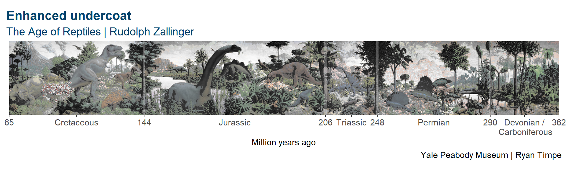
These assumptions provide a rough approximation of the original undercoat. The skies are dark with bright, shadowy clouds. The bodies of all the dinosaurs are visible and the shadowing on Stegosaurus and Allosaurus closely resembles the image of the actual undercoat. The Brontosaurus neck is a bit dark, but for the most part matches the image except for the highlights.
This analysis also makes the low resolution of the image I’m using for analysis more apparent.
Applying these assumptions to the entire mural yields the image below.

These assumptions also perform moderately well for the Permian period, with a dark sail and white body for Edaphodaurus. I’m less impressed with the output in the Cretaceous period, but there is no original to compare it to.
Enhancing the undercoat in the mural
Finally, I wanted to see if increasing the intensity of the undercoat in the original mural would increase the “three-dimensional” effect.
Kinda?
For now, I didn’t manage to completely reproduce the high contrast undercoat of the mural. The original image of Zallinger’s undercoat is bold and detailed, and this reconstruction looks more like a low quality newspaper print.