How To: Spiral line drawings with the tidyverse and gganimate

Convert an image into a single-line spiral drawing using R and the tidyverse.

Note

Originally published on September 11, 2018. Slightly revisited and revised on August 7, 2022.

Introduction

I stumbled on this video from Instagram of an artist creating a picture of Marilyn Monroe by drawing a single spiral from the inside out, varying the thickness of the line to add light and shadow to the image.

Click to watch

After watching the video on loop way too many times, I decided that I had to try and see if could do the same. Given that my drawing skills are near-zero, I turned to R and ggplot. Turns out, this was also a great opportunity to learn Thomas Pedersen’s gganimate package for turning ggplots into animated gifs.

The Goal

Using R, the tidyverse, and gganimate, reproduce a photo as a spiral using just a single line of varying thickness.

Prepare the image

Like the video, we’ll reproduce an iconic black-and-white image, though I chose a portrait of Albert Einstein instead.

As a first step, we resize the image. I had previously written some functions to convert an image into a LEGO mosaic. We can use the scale_image() function from this project, which takes a 3-dimensional JPG or PNG matrix (width, height, RGB channel), crops it into a square, and converts it to a tidy data frame for plotting.

Click here to see script

#1 SCALE IMAGE ----
# Adapted from LEGO mosaics project
scale_image <- function(image, img_size){
  #Convert image to a data frame with RGB values
  img <- bind_rows(
    list(
      (as.data.frame(image[, , 1]) %>% 
         mutate(y=row_number(), channel = "R")),
      (as.data.frame(image[, , 2]) %>% 
         mutate(y=row_number(), channel = "G")),
      (as.data.frame(image[, , 3]) %>% 
         mutate(y=row_number(), channel = "B"))
    )
  ) %>% 
    gather(x, value, -y, -channel) %>% 
    mutate(x = as.numeric(gsub("V", "", x))) %>% 
    spread(channel, value)
  
  img_size <- round(img_size, 0)
  
  #Wide or tall image? Shortest side should be `img_size` pixels
  if(max(img$x) > max(img$y)){
    img_scale_x <-  max(img$x) / max(img$y)
    img_scale_y <- 1
  } else {
    img_scale_x <- 1
    img_scale_y <-  max(img$y) / max(img$x)
  }
  
  #If only 1 img_size value, create a square image
  if(length(img_size) == 1){
    img_size2 <- c(img_size, img_size)
  } else {
    img_size2 <- img_size[1:2]
    img_scale_x <- 1
    img_scale_y <- 1
  }
  
  #Rescale the image
  img2 <- img %>% 
    mutate(y_scaled = (y - min(y))/(max(y)-min(y))*img_size2[2]*img_scale_y + 1,
           x_scaled = (x - min(x))/(max(x)-min(x))*img_size2[1]*img_scale_x + 1) %>% 
    select(-x, -y) %>% 
    group_by(y = ceiling(y_scaled), x = ceiling(x_scaled)) %>% 
    #Get average R, G, B and convert it to hexcolor
    summarize_at(vars(R, G, B), funs(mean(.))) %>% 
    rowwise() %>% 
    mutate(color = rgb(R, G, B)) %>% 
    ungroup() %>% 
    #Center the image
    filter(x <= median(x) + img_size2[1]/2, x > median(x) - img_size2[1]/2,
           y <= median(y) + img_size2[2]/2, y > median(y) - img_size2[2]/2) %>%
    #Flip y
    mutate(y = (max(y) - y) + 1)
  
  out_list <- list()
  out_list[["Img_scaled"]] <- img2
  
  return(out_list)
}

We will want our final spiral to have a radius of 50px (radius), so we can pass radius * 2 to the scaling function, creating a 100 pixel x 100 pixel image.

library(tidyverse)
library(jpeg)

radius <- 50 #pixels
einstein <- readJPEG("Einstein.jpg") %>% 
  scale_image(radius * 2)

einstein$Img_scaled %>% 
  ggplot(aes(x=x, y=y, fill=color)) + 
  geom_raster() +
  scale_fill_identity(guide = FALSE) +
  labs(title = "Scaled Einstein image", 
       subtitle = "100px * 100px") +
  coord_fixed() +
  theme_void()

Polar vs Cartesian coordinates

Drawing a spiral in polar coordinates is easy enough…

tibble(x = rep(c(1:20), 20), y = 1:400) %>% 
  ggplot(aes(x=x, y=y)) +
  geom_path() +
  coord_polar() +
  theme_void()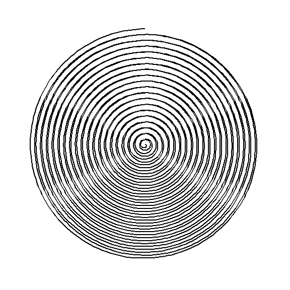

Using that process, I originally tried to convert the image x- and y-values into polar coordinates beginning in the center of the image. That task turned out to be much more difficult than I had imagined.

Instead, I opted to draw a spiral in Cartesian coordinates. It’s been 10 years since my last trigonometry class, but found this helpful post on Stack Overflow. Based off the first answer on the thread, I wrote a function to calculate the points of a spiral centered on the image. All points on this spiral are equidistant, so more points are on the outer sections of the spiral than the inner sections.

Click here to see script

# Function for equidistant points on a spiral

spiral_cartesian <- function(img_df, spiral_radius, num_coils, chord_length, rotation){
  img <- img_df$Img_scaled
  
  #Derive additional spiral specifications
  centerX <- median(img$x)
  centerY <- median(img$y)
  
  thetaMax <- num_coils * 2 * pi
  awayStep <- spiral_radius / thetaMax
  
  #While loop to keep drawing spiral until we hit thetaMax
  spiral <- tibble()
  theta <- chord_length/awayStep
  
  while(theta <= thetaMax){
    #How far away from center
    away = awayStep * theta
    
    #How far around the center
    around = theta + rotation
    
    #Convert 'around' and 'away' to X and Y.
    x = centerX + cos(around) * away
    y = centerY + sin(around) * away
    
    spiral <- spiral %>% 
      bind_rows(tibble(x=x, y=y))
    
    theta = theta + chord_length/away
  }
  
  return(c(img_df, list(spiral = spiral)))
}

We can then pass the einstein image into this function (this provides the function with the desired x- and y-limits), along with specifications for the radius of the spiral (defined earlier), the number of coils, the chord length (distance between each point), and the rotation. We can plot this spiral using coord_fixed() - Cartesian coordinates rather than the polar coordinates above.¹

einstein <- einstein %>% 
  spiral_cartesian(spiral_radius = radius, 
                   num_coils     = 50, #Spiral folds on itself 50 times
                   chord_length  = 2,  #Each point is 2 pixels apart
                   rotation      = 0   #No rotation
                   )

einstein$spiral %>% 
  ggplot(aes(x=x, y=y)) +
  geom_path() +
  coord_fixed() + #Not polar!
  theme_void()

Mapping the image onto the spiral

The artist in the video is able to portray Marilyn Monroe by varying the thickness of the line while drawing a continuous spiral. Now that we have the our spiral in Cartesian coordinates and have scaled it to same size as the photo of Einstein, we need to vary the thickness.

We can do this by effectively overlaying the spiral on top of the image and then assigning the color of the closet image pixel(s) to the spiral point. In this function, I convert the three color channels to an inverted grey scale, where the value of 0 means white, 1 means black, and anything in between is a shade of grey.

Click here to see script

#Project the image onto the spiral
project_image <- function(img_df){
  dat <- img_df$spiral %>% 
    #Round each spiral point to nearest whole number
    mutate(xs = round(x), ys = round(y)) %>% 
    #Join on the rounded points
    left_join(img_df$Img_scaled %>% rename(xs=x, ys=y)) %>% 
    #Create greyscale - 0 is lightest, 1 is darkest
    mutate(grey = R+G+B,
           grey = (1- (grey / max(grey))))
    
  return(c(img_df, list(projected_spiral = dat)))
}

We plot the spiral again, but this time, use the grey value to scale the thickness² of the line. To increase the contrast of the photo, raise the grey value to a power greater than 1.

einstein <- einstein %>% 
  project_image()

einstein$projected_spiral %>% 
  ggplot(aes(x=x, y=y, size = grey^(5/4))) +
  geom_path() +
  scale_size_continuous(range = c(0.1, 1.8), 
                        guide = FALSE) +
  coord_fixed(expand = FALSE) + 
  theme_void()

…Boom! A single spiral of varying line thickness to render an image of Albert Einstein.

Animating the spiral

The original video seems way more impressive than this image. I can’t compete with a hand-drawn image, but can add some drama to this project by animating the spiral, slowly drawing it from the inside out.

We can do this using the package gganimate, which converts ggplots into animated gifs³.

Warning

This post and writing was done with a previous version of gganimate. The tips and script here will need to be updated for the new version.

library(gganimate)

p <- einstein$projected_spiral %>% 
  mutate(row_number = row_number()^(1/2)) %>%  #^(1/2) slows down the beginning of the drawing
  ggplot(aes(x=x, y=y, size = grey)) + #Original contrast for this larger drawing
  geom_path() +
  scale_size_continuous(range = c(0.1, 1.8), 
                        guide = FALSE) +
  coord_fixed(expand = FALSE) + 
  theme_void() +
  transition_reveal(row_number)

Adding gganimate functions to an existing ggplot is simple. We add one new series, row_number, to our data frame, which is used in the final plotting step. Adding + transition_reveal(1, row_number) to the ggplot instructions tells R to render this as an animation, revealing all the data as a single group (1) over the time span row_number. By using the square root of row_number(), gganimate will spend more time drawing the inner sections of the spiral, speeding up as it reaches the outer lines.

Project: ✅ Done

Additional features

The spiral drawing function can be used for color images as well. This doesn’t make much sense for simulating a hand-drawn image using a marker, but still produces a fun image.

goldengirls <- readJPEG("GoldenGirls.jpg") %>% 
  scale_image(radius * 2) %>% 
  spiral_cartesian(spiral_radius = radius, 
                   num_coils     = 50, #Spiral folds on itself 50 times
                   chord_length  = 2,  #Each point is 2 pixels apart
                   rotation      = 0   #No rotation
                   )  %>% 
  project_image()

goldengirls$projected_spiral %>% 
  mutate(row_number = row_number()^(1/2)) %>% 
  ggplot(aes(x=x, y=y, size = grey, 
             color = color)) +
  geom_path(aes(group=1)) + #Add a group to tell it to draw a single line
  scale_size_continuous(range = c(0.1, 1.8), 
                        guide = FALSE) +
  scale_color_identity(guide = FALSE) +
  coord_fixed(expand = FALSE) + 
  theme_void() +
  transition_reveal(1, row_number)

And finally, let’s end where we began, by rendering the image of Marilyn Monroe as an animated spiral.

marilyn <- readJPEG("Marilyn.jpg") %>% 
  scale_image(radius * 2) %>% 
  spiral_cartesian(spiral_radius = radius, 
                   num_coils     = 50, #Spiral folds on itself 50 times
                   chord_length  = 2,  #Each point is 2 pixels apart
                   rotation      = 0   #No rotation
                   )  %>% 
  project_image()

marilyn$projected_spiral %>% 
  mutate(row_number = row_number()^(1/2)) %>% 
  ggplot(aes(x=x, y=y, size = grey)) +
  geom_path() + 
  scale_size_continuous(range = c(0.1, 1.8), 
                        guide = FALSE) +
  coord_fixed(expand = FALSE) + 
  theme_void() +
  transition_reveal(1, row_number)

---

Try it out! Full script can be found on GitHub!

Footnotes

1. The plotted spiral seems to have reflections like a vinyl record. I assume that’s from the rendering of the plot at this resolution.

2. The range values in scale_size_continuous() will require a bit of trial & error and will depend on the final size of the plotted spiral.

3. If you’re using a Windows OS with R 3.5, you might have some trouble installing this package. I recommend reinstalling RTools, referring to this thread, and using this script.